Mathematical description of the Neighbour-Sensing Model
On this page, Audrius Meškauskas, the mathematician who devised the model, guides you through the mathematics on which the Neighbour-Sensing model is based.
Even if you don’t have the mathematical knowledge to appreciate all of the finer points, it’s worth reading through this to get an idea of the number of features that are taken into account, and the way those features are dealt with, to produce this very realistic simulation.
If you would rather study this material on paper than online, an expanded version of this description can be found in our published article, which is available for download as a PDF from the hyperlink in the next information box.
Meškauskas, A., McNulty, L. J. & Moore, D. (2004). Concerted regulation of all hyphal tips generates fungal fruit body structures: experiments with computer visualisations produced by a new mathematical model of hyphal growth. Mycological Research, 108: 341-353. DOWNLOAD a PDF file of the published paper by clicking this hyperlink |
Data representation
Each point and each growth vector contains three components, labelled in this description as px, py and pz. The elementary unit is the hyphal section (symbolised S), defined as a part of the mycelium without branches.
The hyphal section starts at the branch point of the parent section and ends either with the growing tip or with the next branch point (if the section has branched).
The data structure used to describe the section S contains information about the start point (Sfrom), end point (Sto), the growth vector Sgrowth, and a list of the daughter sections (Sbranches).
As a result of the alterations of the growth direction in response to tropic stimuli the section usually has the form of some sort of curve rather than a straight line. To support this, most of the sections also contain a list of internal points (Ssubsegments).
We define n as the total number of sections in the mycelium at the given time t, and
![]()
is the list of sections in the mycelium at the time t.
Field concept
Tropisms and branching regulation are implemented using the field concept. It is supposed that each point of the mycelium generates two types of field. The first type is used to implement a short distance hyphal avoidance reaction and to regulate branching.
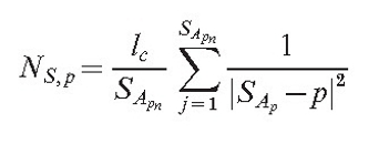
As the field is generated by all points of the mycelium, it is necessary to find a list of points SA (size SApn). This list must be sufficiently large that the averaged field of all its members would be approximately equal to the field of the section. Then the field of the section at the arbitrary point p is:
 |
(3) |
To compute SA, the list {Sfrom} U Ssubsegments U { Sto} is converted into the list of geometrical sections L, where each section connects two adjacent points.
The field of each geometrical section is computed as the averaged field of m equally dispersed points (making set P(m)).
The algorithm exponentially increases m until the field, computed by dividing the section into m points does not differ from the field computed by dividing it into m-1 points by more than the tolerance value e.
After the appropriate m is found, all points from P(m) are added to SA. As can be seen from equation (3), the value of this field is inversely proportional to the square of the distance to the point generating the field. This is true for physical fields such as the electrical or gravitational fields.
Parameter lc is the additional adjustment constant, that makes parameter sets compatible with older versions of the model, where the field was generated only by hyphal tips and branch points. The total field of the mycelium for the point of interest p is then equal to:
|
(4) |
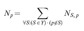
In other words, we suppose that the hyphal section is unable to sense its own field, as that would otherwise contribute an infinite value due to it having zero distance.
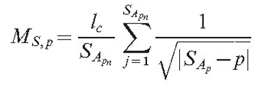
Another type of field (MS,p) is responsible for the long-range interaction. The program allows us to choose between two options:
 |
(5) |
OR
|
(6) |
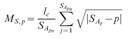
Equation (6) supposes that the field has a stronger value for more remote objects. This may look unusual to the physicist, but it is possible if the field is in reality caused by a chemical that changes as it diffuses. If such a substance is released in an inactive form and slowly changes into an active form while it diffuses, the source can have a stronger impact remotely than it does in its local surroundings. The formula for the total field of the mycelium is identical to equation (4):
|
(7) |
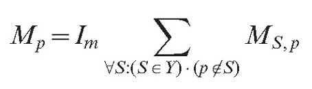
here, Im is the impact factor of the long distance autotropic reaction.
Substrates and other fields
The model space can contain multiple additional objects ('substrates') that generate their own field, causing positive or negative tropisms for the growing cybermycelium. The substrate, T, contains the centre co-ordinates, Tcenter, the radius (TR) and the impact factor (Timpact).
Timpact can be positive or negative (the latter for inhibitory substrates). If needed, all parameters can be interactively altered as the simulation is proceeding. The field of the substrate T is equal to:
|
(8) |
where Ψ is a Heaviside function [a step function, with a value of zero for negative arguments and one for positive arguments]. In other words, the field of substrate is similar to the first type of hyphal field, but Timpact times stronger than the field of the single hyphal segment (length lc). It is equal to zero if the point of interest is inside the substrate.
The field of all substrates at the point of interest p is:
(9) |
We have also implemented a galvanotropic field (a galvanotropism is growth or movement of an organism in response to an electric current). Hyphal segments short enough to be considered straight lines form the galvanotropic orientation field. This field is directed towards the end of the segment that is closest to the corresponding hyphal tip and is parallel to the hyphal axis. The absolute value of the field at any given point is inversely proportional to the shortest distance from that point to the segment generating the field. The total field of the mycelium (which we symbolise vc) at any given point is a vector sum of all the fields generated by all such hyphal segments.
Defining the galvanotropic field allows two new types of tropism to be introduced. The first is a parallel tropism that directs the growing hyphae to turn into the same direction of growth. This is an effective way of co-ordinating the growth of several hyphae into a strand or cord. The second orients hyphae perpendicularly to vc, and can be used as an alternative or replacement for the previously mentioned positive and negative autotropisms.
Although these field equations do not require that the active agent is an electric field (but merely something that behaves like an electric field), it may well be biologically accurate in view of the fact that the accumulation of many nutrients into live hyphae is driven by proton gradients maintained by transporters in the membrane. In living fungi these 'proton pumps' tend to be polarised along the hypha by being concentrated in regions of active growth adjacent to the hyphal apex.
Finally, to produce polarized structures, like mushroom fruit bodies, we introduced the concept of the orientation field. In contrast to the previous fields, this is a directional field, oriented in the direction of the z axis of the modelling space. The hyphae can try to grow by any arbitrary chosen angle β Î[0…180°] in relation to the vector of this field.
Growth simulation
Fields, defined by equations (3), (6) and (9) are scalar, and growth can be directed towards or against their gradient. All these equations can be differentiated with respect to px, py and pz, obtaining the values for the field gradient vector at the point p (we used the program ‘Maple’ for differentiation and code generation).
If several field concepts are used, we obtain several field gradients. To facilitate analysis, the gradient vectors can be displayed next to the growing hyphal tips. Then, the current orientation of the cumulative tropism vector for the section S is:
Equation (10) |
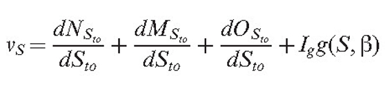
where
|
(11) |
and differentiation with relation to the point p = Sto means differentiation with relation to px for the vector component x, etc.
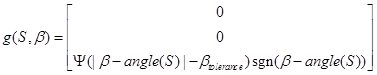
The function g defines the impact of the orientation field and the model parameter Ig; the impact of this tropism on the orientation and angle (S) is the tip orientation angle for the section S. Equation (11) incorporates a tolerance angle βtolerance to avoid the tip hunting around the optimum.
The growth vector of the section is updated in the following way:
Equation (12) |
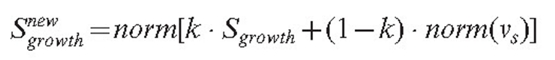
where
|
In equation (12), the parameter k defines a coefficient of persistence, which is used to ensure that branches change direction gradually; and it operates on the previous growth vector Sgrowth.
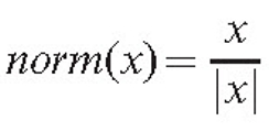
The function norm(x) ensures that the density gradient alters the direction but not the speed of the growth. Otherwise, a high gradient, if formed accidentally, would cause unreliably fast growth in some parts of the mycelium. The position of the tip is updated, the new value being equal to:
|

where a is the model parameter defining the growth rate. In the current version of the model, growth is only possible if the hyphal section is terminated with an unbranched hyphal tip.
Vector rotation
Interesting results can be obtained if the tropism vectors ![]() and g(S, β) are rotated around the hyphal axis before using them for modification of the growth vector.
and g(S, β) are rotated around the hyphal axis before using them for modification of the growth vector.
The model allows rotation of these vectors by an arbitrary angle, applying the known formulas for vector rotation. Rotation of the vector of the autotropic reaction can cause curling of the growing tip around the other hyphae. Rotation of the gravitropic vector may form spiral structures within the mycelium.
Branching
In our model, branch initiation is controlled by two steps. In the first step, the branching condition is checked. Depending on the experimenter’s choice, this condition can be either of the following:
|
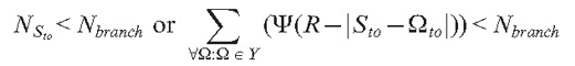
Nbranch is the model parameter defining either the number of neighbouring tips in the sphere of radius R or the threshold value of the density field.
In the next step, a random uniformly distributed number (r) is generated such that rÎ[0…100] and branching is initiated if r < pbranch.
The parameter pbranch defines the branching probability during one iteration if the initial branching condition is satisfied.
Formally the section branches into two branches, but one of them (the primary) obtains a copy of the growth vector of the parent branch, continuing in the same direction.
Depending on the user-modifiable settings, the other (secondary) branch can be oriented randomly or adjusted to follow the direction of the tropic vector at the point of branching. Sfrom and Sto values of the both new branches are initialized to the Sto value of the parent branch.
Age and length limitations
The branching condition can be extended, allowing branching only for sections whose ages do not exceed the given limit. Similarly, it is possible to set the age and length limit for branch growth. To implement these features, each section contains two additional fields, Sage and Slength. During each iteration, Sage is incremented by 1 and Slength is incremented by a.
Describing mycelia and parameters in XML ... and the days before multi-core tablets and phones ...
Data defined in the XML language consists of multiple tags, each having a name, associated parameters and possibly other, nested tags. As the tags can be accessed by name, introducing new tags does not make the previously stored data files incompatible as long as the default values of these new tags are known.
Hence XML is a good language for defining the model parameters, as the number of parameters rapidly increases during program development. We also used the same XML file to store details about all placed substrates and all sections of mycelium.
XML stands for eXtensible Markup Language. XML was designed to store and transport data, and to be both human- and machine-readable [see the XML Tutorial at W3schools.com CLICK HERE to open this website in a new window]. |
When the parameter tags only occur once per file, the <section> tag is repeated for each section of mycelia, and the <substrate> tag is repeated for each substrate. This strategy was initiated when the programs were first developed because of the limited processing power of the then-available single-core desktop PCs. Such combined parameter-data files could be created on a desktop PC and later started on a multi-processor supercomputer, where batch mode was usually preferred and direct interaction with the user during execution was not always possible. Supercomputers generated the analogous XML file that could then be reloaded to the desktop PC for viewing the results, modifying some parameters and possibly returning to the supercomputer for continuation. Being human-readable, XML also allows the experimenter to see the exact definitions of each section of mycelia.
As each of several hundreds of hyphal tips is driven by exactly the same algorithm, at the time the task seemed to be ideal for parallel execution on a multi-processor supercomputer. However, the first runs on a large number of processors showed much poorer performance than was expected. Detailed analysis of the problem revealed that processors, despite being equally loaded, spent significant time in a waiting mode because all processors needed to access information about all sections of mycelia. The amount of this information can be up to several megabytes, and it must be renewed for each iteration. Unfortunately, the Java virtual machine was unable to ensure effective sharing of the data in this case, taking much more time than it should need to transfer information between processors. Our programs were used to investigate the root cause of this problem.
For our work, we tried to reduce the information stream by transferring only differences as the majority of the mycelium points do not change between iterations. This improved parallel execution performance by a factor of approximately two, making it really worthwhile to run tasks on a multiprocessor machine rather than on a desktop computer.
These inefficiencies are no longer an issue as multi-core processors in today's PCs have efficient data flow management built-in.
The program will save snapshot views of the simulation as it runs. These checkpoints are saved as XML files. The default arrangement is for XML files to be saved after each 10 iterations (that is at 10 program time unit intervals). The timing can be adjusted by the user (saving XMLs every 50 iterations is useful for logging the progress of complex visualisations on an untended computer). These XML files can be used to store simulations, to restart simulations, and to generate JPG graphics and animations (the latter being made from sequences of the JPG files using a suitable shareware video maker).
Copyright © David Moore 2017