Liam McNulty takes you through some experiments with the Neighbour-Sensing model of mycelial growth
This page summarises a series of experiments that explore some of the capabilities of the Neighbour-Sensing model.
I spent some weeks over the summer of 2003 systematically exploring the model by changing parameters and saving the resultant images of mycelia as jpeg files. What follows is a formal record of these experiments. The experiments were done by changing the parameters that the simulation uses in its mathematical computations, so that you can SEE on screen the effects of those parameters on growth of the cyberfungus. CLICK HERE to download a PDF version of this guide into a new window.
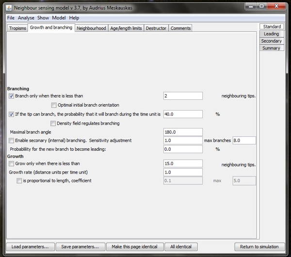 |
| One of the user interface screens of the Neighbour-Sensing program which is used to set the parameters for each run of the program. The 'parameters are set' by ticking the check boxes at extreme left to choose the major characteristics required in the experimental mycelium. The user then enters numerical values in the edit boxes on the right hand side of the form in order to define the values of those parameters. Note that the time unit (referred to under 'Growth rate' is equal to 300 milliseconds. |
What follows in this document is a record of these experiments presented in tabulated form standardised so that the upper cell shows the image of the mycelium generated by the parameter set which is listed in the legend in the lower cell. Unused parameters are simply not mentioned, but parameter(s) shown in red-bold font are the ones being experimented with in that simulation.
The time units shown at the start of each parameter set should be viewed as consecutive blocks during which that parameter set has been operative. Each figure has a standard scale bar of 100 length units. Simulations can be paused, parameters changed, and the simulation resumed. In these cases several parameter set lists are shown accompanying a single illustration. Note also that all the images of cybermycelia have small circles at the ends of branches; these are tags that identify the position of the 'growing' apex, in images derived from on-screen simulations they are colour-coded red for non-growing and blue for growing tips in the algorithm iteration which is displayed.
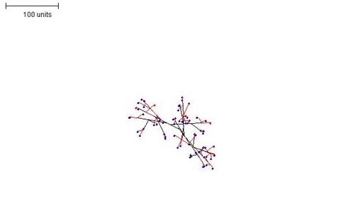
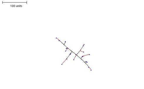
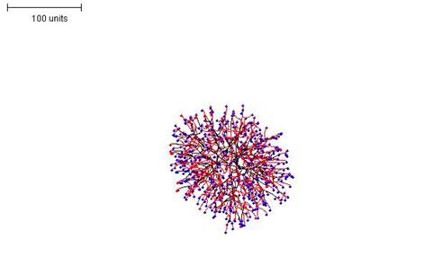
Figures 1-3 show the effects of varying the autotropism setting.
 |
| Figure 1. Growth pattern without negative autotropism. Parameters: 100 time units; no negative autotropism; branch only when less than 3; grow only when less than 15 neighbouring tips in radius = 20; branching probability = 40; growth speed = 1. |
 |
| Figure 2. Growth pattern with negative autotropism implemented at a value of 0.5. 100 time units; with negative autotropism at 0.5; branch only when less than 3; grow only when less than 15 neighbouring tips in radius = 20; branching probability = 40; growth speed = 1. |
 |
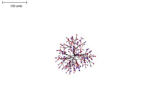
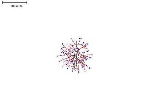
| Figure 3. Growth pattern with negative autotropism set to 0.1. 100 time units; with negative autotropism at 0.1; branch only when less than 3; grow only when less than 15 neighbouring tips in radius = 20; branching probability = 40; growth speed = 1. |
Figure 3 shows the growth pattern obtained with negative autotropism set to 0.1. This seems to produce the most realistic mycelial shapes and was the value used in most of the subsequent examples shown here.
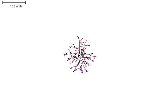
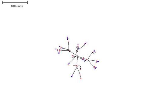
Figures 4 and 5 illustrate growth patterns produced with different levels of control over the probability of branching (but with the same growth rules).
 |
| Figure 4. Growth pattern obtained by setting a low threshold for preventing branching i.e. making branching rare) (compare with Figure 5). 100 time units; with negative autotropism at 0.1; branch only when less than 2 neighbouring tips in radius = 20; branching probability = 40; growth speed = 1. |
 |
| Figure 5.Raising the threshold for preventing branching (that is, making branching more frequent) results in a much denser mycelial structure (compare with Figure 4). 100 time units; with negative autotropism at 0.1; branch only when less than 8 neighbouring tips in radius = 20; branching probability = 40; growth speed = 1. |
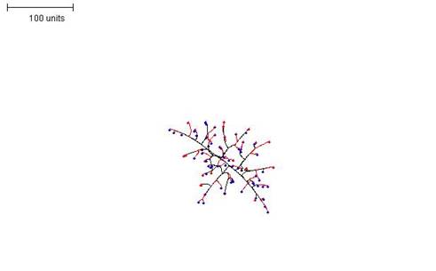
Introducing a limitation on the growth of tips modifies the colony morphology further, resulting in a structure of intermediate density (Figure 6). However, if this parameter is implemented its value must be larger than that of the branching threshold parameter for a growing mycelium to result.
 |
| Figure 6. Making the growth of hyphal tips depend on the number of hyphal tips in the neighbourhood. Branching rule the same as in Figure 5. 100 time units; with negative autotropism at 0.1; branch only when less than 8; grow only when less than 15 neighbouring tips in radius = 20; branching probability = 40; growth speed = 1. |
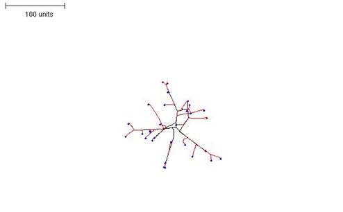
Interestingly, a similar effect to decreasing the threshold for preventing branching and growth can also be achieved by increasing the radius that defines ‘neighbouring tips’. In this scenario, a sparser structure is produced with longer segments of hyphae before branching is initiated (Figure 7); note that the longer segments do not result from an increase in filament growth rate, which remains set at 'growth speed = 1'.
 |
| Figure 7. Increasing the radius that defines the neighbourhood. Growth and branching rules otherwise the same as in Figure 6. 100 time units; with negative autotropism at 0.1; branch only when less than 8; grow only when less than 15 neighbouring tips in radius = 40; branching probability = 40; growth speed = 1. |
The above examples show some of the morphological variation that can be achieved by altering parameters for a single simulation. But simulations can be paused, and the pause allows parameter sets to be changed so that the simulation proceeds under a new set of rules when it is resumed. By switching between parameter sets like this, it is possible to produce more complex mycelial structures. In the example shown in Figure 8 three stages were employed:
- first, a parameter set was chosen that produces a dense mycelium, and this was operated for 100 time units;
- second, the simulation was paused and the growth threshold and the size of the radius defining the neighbouring tips were adjusted so that only a few tips continued growth. Furthermore, the probability of branching was reduced to a value close to zero. These settings were operated for a further 200 time units, and then paused again;
- finally, a parameter set that produces a dense globular outgrowth of tips was implemented (for 50 time units). Note that the definition of neighbouring tips is kept large in this parameter set so that tips in the original ‘parent’ mycelium do not resume growth.
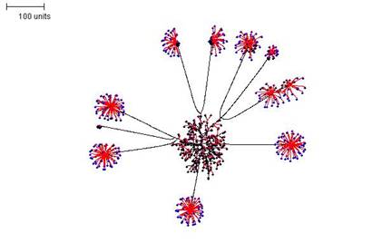 |
| Figure 8. Compound mycelial structure produced by pausing the simulation, changing the parameter settings, and then resuming 'growth'. Parameter set 1: 100 time units; with negative autotropism at 0.1; branch only when less than 8; grow only when less than 15 neighbouring tips in radius = 20; branching probability = 40; growth speed = 1. Parameter set 2: 200 time units; with negative autotropism at 0.1; grow only when less than 150 neighbouring tips in radius = 75; branching probability = 0.1; growth speed = 1. Parameter set 3: 50 time units; with negative autotropism at 0.1; branch only when less than 100; grow only when less than 150 neighbouring tips in radius = 100; branching probability = 80; growth speed = 1. |
The compound mycelium illustrated in Figure 8 is very reminiscent of a mycelium producing sporophores tipped with bundles of spores of the sort that can be formed by so many different filamentous fungi. In biological terms we imagine the 'pause simulation and change parameters' in the modelling process to be equivalent to a change in conditions (either environmental, like temperature, illumination, availability of nutrients, etc., or intracellular, such as the availability of nutrient stores, like glycogen, or levels of regulatory molecules, like cyclic-AMP) that initiate a different pathway of differentiation.
Most parameter settings generate spherical colonies, and that includes a setting in which all controls are removed and growth and branching depend on randomised 'decisions'. In other words, the basic spherical (circular in projection) morphology of the fungal colony arises without the need for global control of that morphology. However, the program does not limit us to spherical end-points.
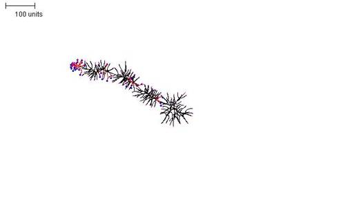
A thin filament (Figure 9) can be formed by setting the parameters that prevent growth and branching to high thresholds (i.e. the growth and branching of tips is made highly probable), but then limiting the time for which the tips can grow and branch. There are two ways to limit the length of branches: first, by limiting the time allowed for their growth; and second, by limiting the length to which the segments are allowed to grow. Both strategies have the same effect.
To create a number of tips from which the filament can extend, any parameter set can be used that generates reasonably large numbers of tips per time unit.
 |
| Figure 9. A parameter set that generates a sparsely-branched filament. First 10 time units: use any parameter set that generates reasonably large numbers of tips per time unit. For the next 250 time units: with negative autotropism at 0.1; branch only when less than 10; grow only when less than 20 neighbouring tips in radius = 20; stop growing after tip = 10; stop branching after tip = 10; branching probability = 80; growth speed = 1. |
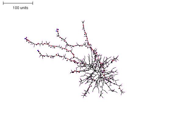
A more prolifically-branched filament can be produced (Figure 10) by increasing the threshold for preventing branching and growth (i.e. increasing the density of branches) and by allowing the tips to branch and grow for longer. The branching probability can also be increased to accentuate the effect.
 |
| Figure 10. A parameter set that generates a densely-branched filament. For the first 30 time units use any parameter set that generates reasonably large numbers of tips per time unit. For the next 300 time units: with negative autotropism at 0.1; branch only when less than 80; grow only when less than 120 neighbouring tips in radius = 80; stop growing after tip = 30; stop branching after tip = 30; branching probability = 80; growth speed = 1. |
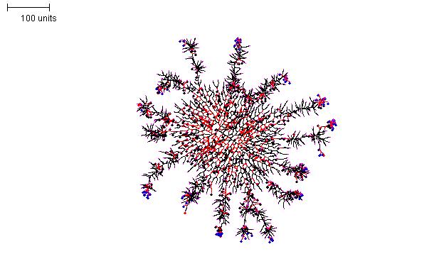
Increasing the time that the initial parameter set is run at the start, and then switching to a thin filament parameter set can produce a globular structure with thin ‘exploratory’ filaments emanating from it (Figure 11).
 |
| Figure 11. Creating exploratory filaments emerging from a spherical mycelium. For the first 100 time units use any parameter set that generates reasonably large numbers of hyphal tips per time unit. In the next 200 time units: use negative autotropism at 0.1; branch only when less than 8; grow only when less than 15 neighbouring tips in radius = 20; stop growing after tip = 10; stop branching after tip = 10; branching probability = 80; growth speed = 1. |
Implementing the density field hypothesis for branching regulation represents a slightly different way of calculating the density of tips in the locality. The main practical difference between this form of computation and that in the examples discussed above is that when the density field is used, local differentiation becomes difficult as the regulation applies to the whole mycelium.
For instance, the structure illustrated in Figure 8 would be impossible using this method, as it cannot prevent growth and branching in the ‘parent’ mycelium while allowing it in the ‘daughters’. Thus, structures are produced that are uniformly distributed with branches, and most branching appears to be dichotomous. Figure 12 shows three examples in which the density field threshold for branching was varied to produce mycelia with different morphologies.
 |
| Figure 12A. 100 time units; with negative autotropism at 0.1; using density field hypothesis, branch if field is less than 0.1; branching probability = 40; growth speed = 1. |
 |
| Figure 12B. 100 time units; with negative autotropism at 0.1; with density field hypothesis, branch if field is less than 0.05; branching probability = 40; growth speed = 1. |
 |
| Figure 12C. 100 time units; with negative autotropism at 0.1; density field hypothesis, branch if field is less than 0.01; branching probability = 40; growth speed = 1. |
| Figure 12. Three examples in which the density field threshold for branching was varied to produce mycelia with different morphologies. |
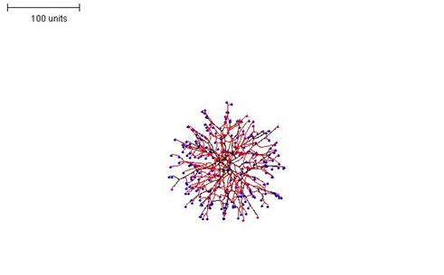
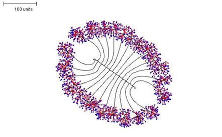
If negative autotropism is set to zero at the beginning of the simulation (switching this parameter to zero during a simulation produces different results) an interesting growth process can be seen. This can be done with both methods of branching regulation, but the density field hypothesis is used in the examples shown here. The interesting feature of the growth of these mycelia is that they grow in one plane at a time. That is to say, a straight, single hypha grows first with many dormant tips along it; then branches grow perpendicularly to produce a 2-dimensional disc-type structure; and finally more branches grow out perpendicularly from that to make a 3-dimensional structure. If a relatively high density field threshold is used, an ellipsoidal morphology is produced (Figure 13).
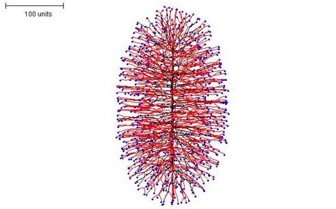 |
| Figure 13. Ellipsoidal morphology. 100 time units; with negative autotropism set to zero; with density field hypothesis, branch if field is less than 0.1: branching probability = 80; growth speed = 1. |
If the density field threshold is reduced greatly, the result is a rod-like structure (Figure 14).
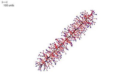 |
| Figure 14. Rod-like morphology. 100 time units; with negative autotropism at zero; with density field hypothesis, branch if field is less than 0.005; branching probability = 80; growth speed = 1. |
Again, switching between parameter sets in the course of a simulation generates interesting compound morphologies. For Figure 15, three parameter sets were used in sequence:
- First, negative autotropism was set to zero and the density field hypothesis used, with the threshold for branching set reasonably high (i.e. branching is likely). This produces a short, straight hypha with many (dormant) tips in 90 time units.
- Second, once the tips on the hypha begin to extend perpendicularly, the branching threshold and probability are lowered so that long branches are grown for 110 time units.
- Finally, the branching threshold and probability are raised to very high values and the tip growth is limited to 25 time units. This causes dense branching around the growing tips.
 |
| Figure 15. Compound morphology produced by three successive parameter sets using regulation by the hyphal density field. Parameter set 1: 90 time units; using negative autotropism set to zero; with density field, branch if field is less than 0.1; branching probability = 80; growth speed = 1. Parameter set 2: 110 time units; with negative autotropism set to zero; with density field, branch if field is less than 0.005; stop branching after tip = 50; branching probability = 20; growth speed = 1. Parameter set 3: 25 time units; with negative autotropism set to zero; with density field, branch if field is less than 0.5; stop growing after tip = 25; branching probability = 80; growth speed = 1. |
For the structure shown in Figure 16, an ellipsoid mycelium, as described in Figure 14, was grown initially for 200 time units. Then the parameters were switched to a set that produces densely branched filaments (as in Figure 10) for a further 100 time units.
 |
| Figure 16. Compound morphology produced by two successive parameter sets. Parameter set 1: 200 time units; with negative autotropism set to zero; with density field, branch if field is less than 0.1; branching probability = 80; growth speed = 1. Parameter set 2: 100 time units; with negative autotropism at 0.1; branch only when there are less than 50 neighbouring tips; grow only when there are less than 80 neighbouring tips in radius = 50; stop growing after tip = 20; stop branching after tip = 20; branching probability = 80; growth speed = 1. |
We will be looking at a range of more complex examples in the next page, but before doing so it’s worth restating that the essential element of the Neighbour-Sensing model is a cyberhyphal tip that has four characteristics:
- position in three-dimensional space;
- a growth vector;
- length;
- ability to branch.
During each iteration of the algorithm the tip advances by a growth vector (initially set by the user) in accordance with the effects of one or more tropic vectors, and may branch (with an initial probability set by the user), branching also in accordance with the effects of one or more tropisms set by the user. That’s all. The patterns you can see in the above examples emerge from application of the rules that govern these simple characteristics.
Now, go to the next page for some more unexpected surprises ...
Read on!
Copyright © David Moore 2017